Tutorial
The following tutorial follows the typical work-flow analyzing an eNMR measurement. Code marked with >>> is input code, while all other lines are the respective output.
Importing and processing the eNMR spectrum
loading the data
Loading the eNMR data takes place by creating an instance (object) of the respective import class with the respective path and expno of the experiment. This is the most critical point when adapting a different experimental setup to eNMRpy. If you are in need for help, please consider a pull request on GitHub.
>>> import eNMRpy
>>> m = eNMRpy.Import_eNMR_Measurement(path, expno, dependency='U', lineb=.5, d=2.2e-2, cell_resistance=None)
Processing the spectrum (FFT, linebroadening)
Usually, the imported data represents the free induction decay (FID), recorded for the eNMR measurements. In order to analyze the eNMR measurement, the FID needs to be transformed into a spectrum via Fast Fourier Transformation (FFT) via the .proc() method.
>>> m.proc(linebroadening=None, phc0=0, phc1=0, xmin=None, xmax=None)
This method transforms the self.data array from the FID to the spectrum. phc0 and phc1 give the zero and first order phase correction. If xmin and/or xmin are not None, self.set_spectral_region() will be called with the given limits.
Note: Please keep in mind, that self.data is changed. It should always be used directly after loading the raw data. Therefore, it is good practice to write self.proc() in the same cell within a jupyter notebook, in order to obtain the correct spectrum after each execution of the respective cell.
Plotting the spectrum
After loading the raw data, and processing the spectrum, we want to have a look at the result by plotting the spectrum via the method self.plot_spec(). This method returns a matplotlib figure, which can be used as usual. The first argument in self.plot_spec() can be an integer or an array of integers, in order to plot multiple rows of the 2D spectrum on top of each other.
>>> fullspec = m.plot_spec(rows, figsize=(x,y));
Important instance variables
| variable | meaning |
|---|---|
| self.eNMRraw | contains the phase data, voltage list, and gradient list data for all eNMR experiments |
| self.d | electrode distance in m (cell constant) |
| self.Delta | observation time in s |
| self.delta | magnetic field gradient pulse duration |
| self.gamma | gyromagnetic ratio in °/Ts |
| self.path | path used to import the data |
| self.expno | experiment number according to Bruker’s syntax |
| self.lineb | line broadening variable used for processing |
| self.ppm | list of chemical shift for each datapoint |
| self.data | 2D numpy array containing the complex spectral data |
| self.nuc | investigated nucleus |
| self.title_page | imported title page from bruker file -> transformed to be used with print |
| self.dependency | voltage, gradient, or current dependent measurement –> see docstring |
| self.cell_resistance | important to calculate the electric field when const. I mode is used |
Phase analysis
eNMRpy comes with three different methods for the determination of the electrophoretic mobility. a) Fitting of Lorentzians, b) automatic phase correction, and c) Mobility Ordered SpectroscopY (MOSY). A brief description of all these methods can be found in the linked open access article published in Magnetic Resonance in Chemistry by Wiley.
Approximation of Lorentzian-shaped function
In order to analyze the phase shift via the approximation of Lorentzian shaped profiles, one has to import the submodule Phasefitting accordingly:
>>> from eNMRpy import Phasefitting as phf
Two methods exist for the creation of the lmfit fit model.
Peak picking
The first model uses the peakpicker() function contained in the Phasefitting module to obtain an array (in this example peaks) listing the peaks picked. The peakpicker() function needs the x-coordinate (m.ppm) and y-coordinate (here the first spectral row m.data[0] of the measurement object m), and a threshold below which no peak is picked:
>>> peaks = phf.peakpicker(m.ppm, m.data[0], threshold=1e5)
Peak selection via GUI
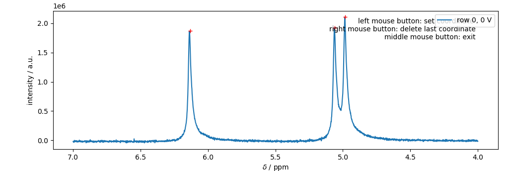
Since the peak picking approach is not always reliable, one can use a GUI for the selection of the individual peaks.
>>> %matplotlib  qt5          # enables matplotlib to open a GUI outside of the jupyter notebook
>>> peaks = phf.set_peaks(m)  # starts the GUI
>>> %matplotlib inline        # returns to the inline-plotting mode for the jupyter notebook
Peaks are selected by a left-click, the last peak can be deleted via a right-click. Note: that the red crosses correspond to the clicking points, where the peaks were selected. This is important for estimating the peak’s amplitude. Note: It is important to close the GUI by either clicking the middle bouse button, or pressing <enter> on the keyboard. Otherwise, the jupyter notebook may be stuck in a while loop.
Creating the fit model and fitting the eNMR measurement
The peaks array, obtained via one of the two methods described above, is then passed to the make_model() wrapper function, returning an instance of the lmfit.Model()-class (named model in this example) including the correct parameters set, and Lorentzian function.
>>> model = phf.make_model(peaks, print_params=False)
A key aspect of the fitting method is to introduce physically meaningful restrictions to the fitmodel by defining dependencies between parameters. The most straightforward restriction is to set signal phases corresponding to the same molecule equal by using the method self.set_mathematical_constraints(). In this example, ph0 = ph1 = ph2 hence, only ph2 is varied in the following fit. (see self.params.pretty_print())
>>> model.set_mathematical_constraints(['ph0=ph1', 'ph1=ph2'])
The set of parameter can be investigated via:
>>> model.params.pretty_print()
Name         Value      Min      Max   Stderr     Vary     Expr Brute_Step
a0        2.107e+04        0      inf     None     True     None     None
a1        1.927e+04        0      inf     None     True     None     None
a2        1.867e+04        0      inf     None     True     None     None
baseline         1     -inf      inf     None     True     None     None
l0            0.01        0      inf     None     True     None     None
l1            0.01        0      inf     None     True     None     None
l2            0.01        0      inf     None     True     None     None
ph0              1     -180      180     None    False      ph1     None
ph1              1     -180      180     None    False      ph2     None
ph2              1     -180      180     None     True     None     None
v0           4.985     -inf      inf     None     True     None     None
v1           5.063     -inf      inf     None     True     None     None
v2           6.137     -inf      inf     None     True     None     None
Furthermore, it is possible to manipulate single parameters according to the documentation of the lmfit package.
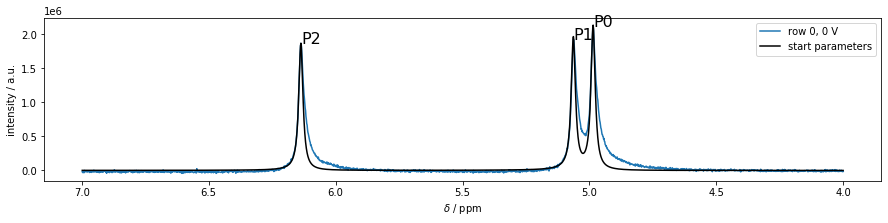
The initial spectrum can be plotted via model.plot_init_spec(), which takes the x-coordinate m.ppm and as an optional argument the 1D figure fullspec
>>> fullspec = m.plot_spec(0);
>>> model.plot_init_spec(m.ppm, fig=fullspec);
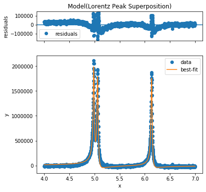
In order to see, whether the initial parameters are well-chosen resulting in a converging fit, a test-fit of the first spectrum can be achieved using the self.fit() method of the fit-model:
>>> model.fit(m.ppm, m.data[0], plot=True);
In order to fit a whole eNMR measurement, the function Phasefitting.fit_Measurement() is used inserting the measurement object m, and the fit model model. Using this function, all eNMR spectra in m are fitted consecutively, and the results are stored in the m.eNMRraw pandas-DataFrame.
>>> phf.fit_Measurement(m, model, plot=False, parse_complex='real')
The results of the fit can be found in the measurement objects eNMRraw pandas DataFrame. In this example m.eNMRraw.
Automatic phase correction
A simple way to analyze the phase shift is the analysis via zero order phase correction. Here, a very straight forward phase correction algorithm described earlier is employed. The implementation of this method was adapted from the nmrglue package and altered in order to match the scope of this work.
The method self.autophase_phase_analysis() is executed, and automatically starts the analysis while storing the results in the self.eNMRraw pandas-DataFrame in the “ph0acme” column.
>>> m.autophase_phase_analysis()
Note: This method is a quick analysis which is only applicable to spectra exhibiting resonances of a single substance, where no superposition of signals with different phase shifts is expected.
Mobility Ordered SpectroscopY MOSY
MOSY is a 2D Fouriertransformation-based technique for the analysis of the electrophoretic mobility \(\mu\), where the signal intensity is described via
In order to perform the fourier transformation, the module MOSY has to be imported, the mosy object is created from the MOSY.MOSY()-class, and processed via the self.calc_MOSY()-method
>>> from eNMRpy import MOSY
>>> mosy = MOSY.MOSY(m)
>>> mosy.calc_MOSY()
zero filling started!
(11, 1967) (4096, 1967)
zero filling finished!
done
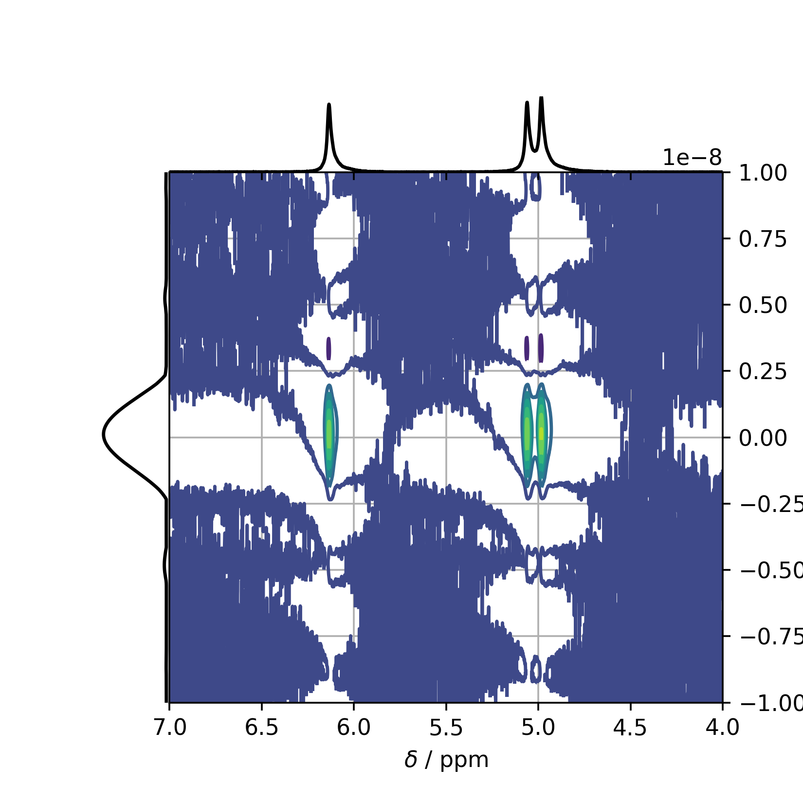
In order to view the result, the method self.plot_MOSY() can be used returning a matplotlib figure named mosyfig in this example. Note: The xlim is set in from high to low values, as it is common in NMR spectroscopy.
>>> mosyfig = mosy.plot_MOSY(xlim=(7,4))
This plot results in the following figure showing the full spectrum, including truncation artifacts etc.:
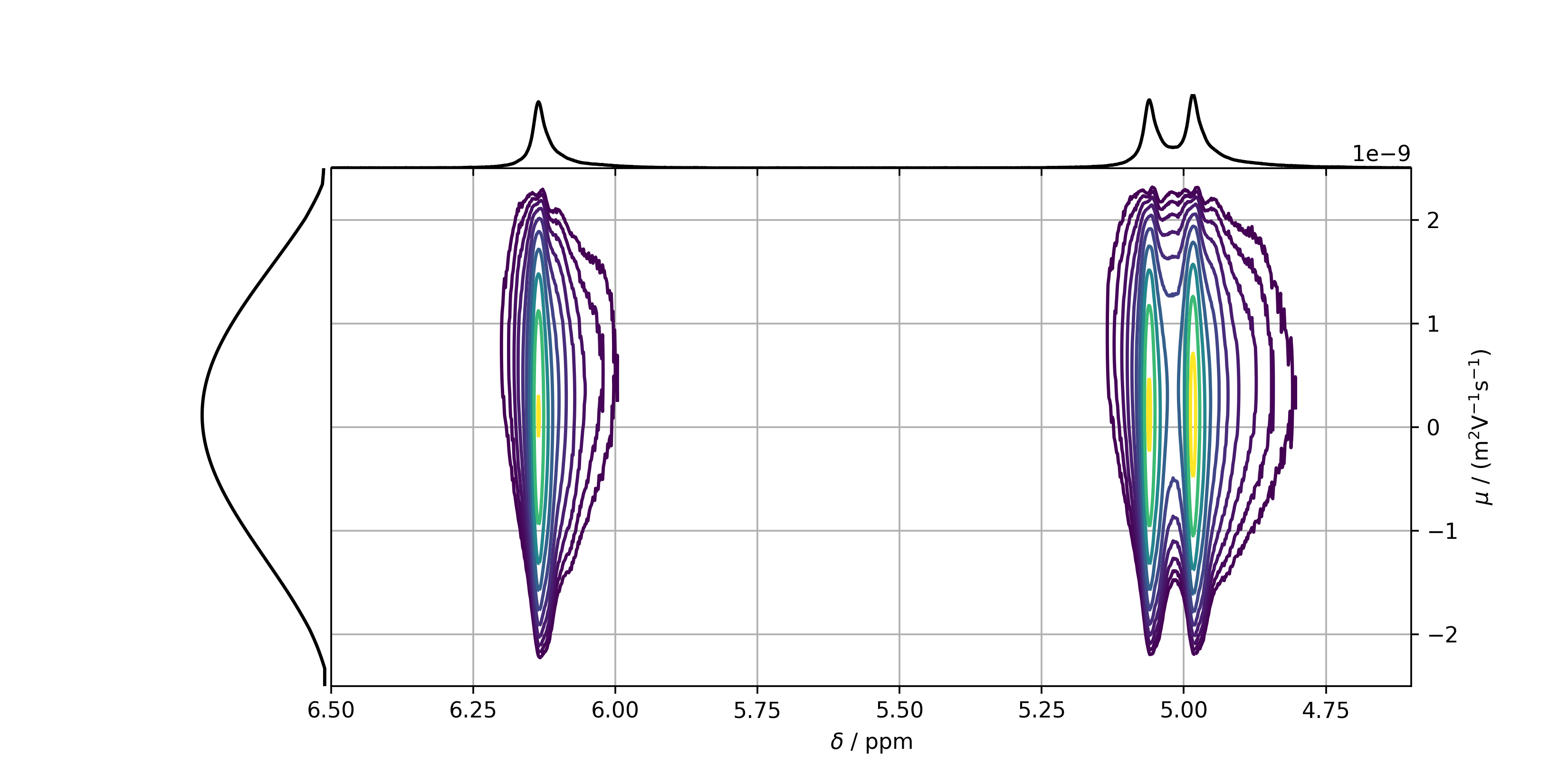
In order to clean up the MOSY spectrum, one can rescale the figure accordingly:
>>> import numpy as np

>>> zoom = 1e6
>>> base = 1.39 #changes the distance of the lines -- base of the exponential term
>>> number_of_lines = 10

>>> mosyfig = mosy.plot_MOSY(xlim=(6.5,4.6), ylim=(-2.5e-9, 2.5e-9), figsize=(10,5),
>>>                          levels=zoom*base**np.linspace(0,10,number_of_lines))
Leading to the following figure:
In order to determine the position of the peaks, and therefore the mobility, it is recommended to plot slices in the mobility domain of the peaks on top of each other. For this reason, a list containing the chemical shifts of the peaks is necessary. This list can either be created manually, or by using the automatic peakpicker tool, or the GUI explained above.
>>> from eNMRpy.Phasefitting import peakpicker
>>> peaks = peakpicker(m.ppm, m.data[0]) # list of peaks with [[ppm, intensity],..].
>>> slices_ppm = peaks[:,0]              # Only chemical shifts are returned from peaks via peaks[:,0]
The figure containing the MOSY slices is then created via the self.plot_slices_F1() method.
mosyslicefig = mosy.plot_slices_F1(slices_ppm)
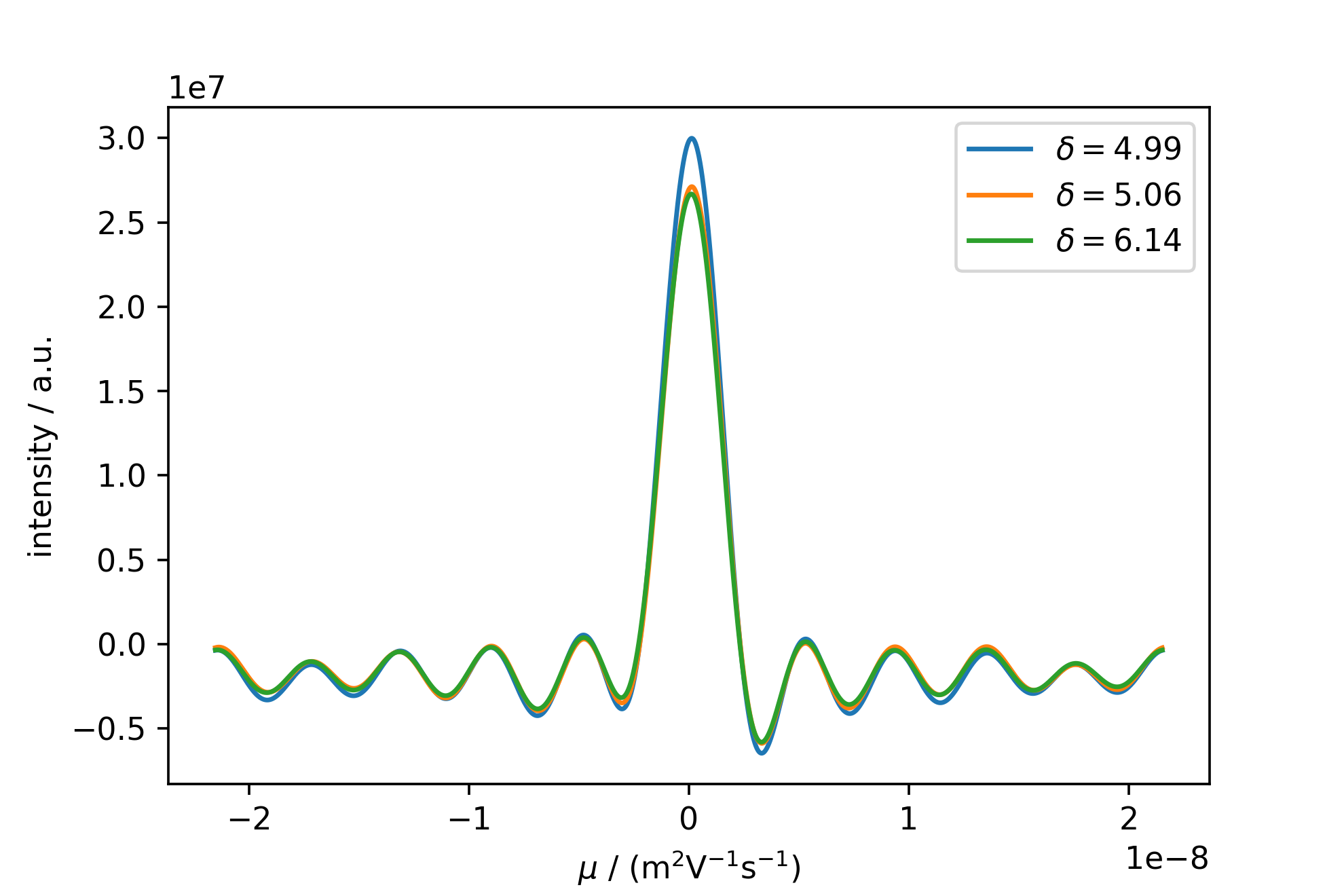
This figure shows the strong sync-modulation originating from a truncated FID and FFT in the mobility dimension. Rescaling the image, and autopicking and annotating the peaks with their respective mobility yields the following:
mosyslicefig = mosy.plot_slices_F1(peaks[:,0], xlim =(-2.5e-9, 2.5e-9) ,annotate=True)
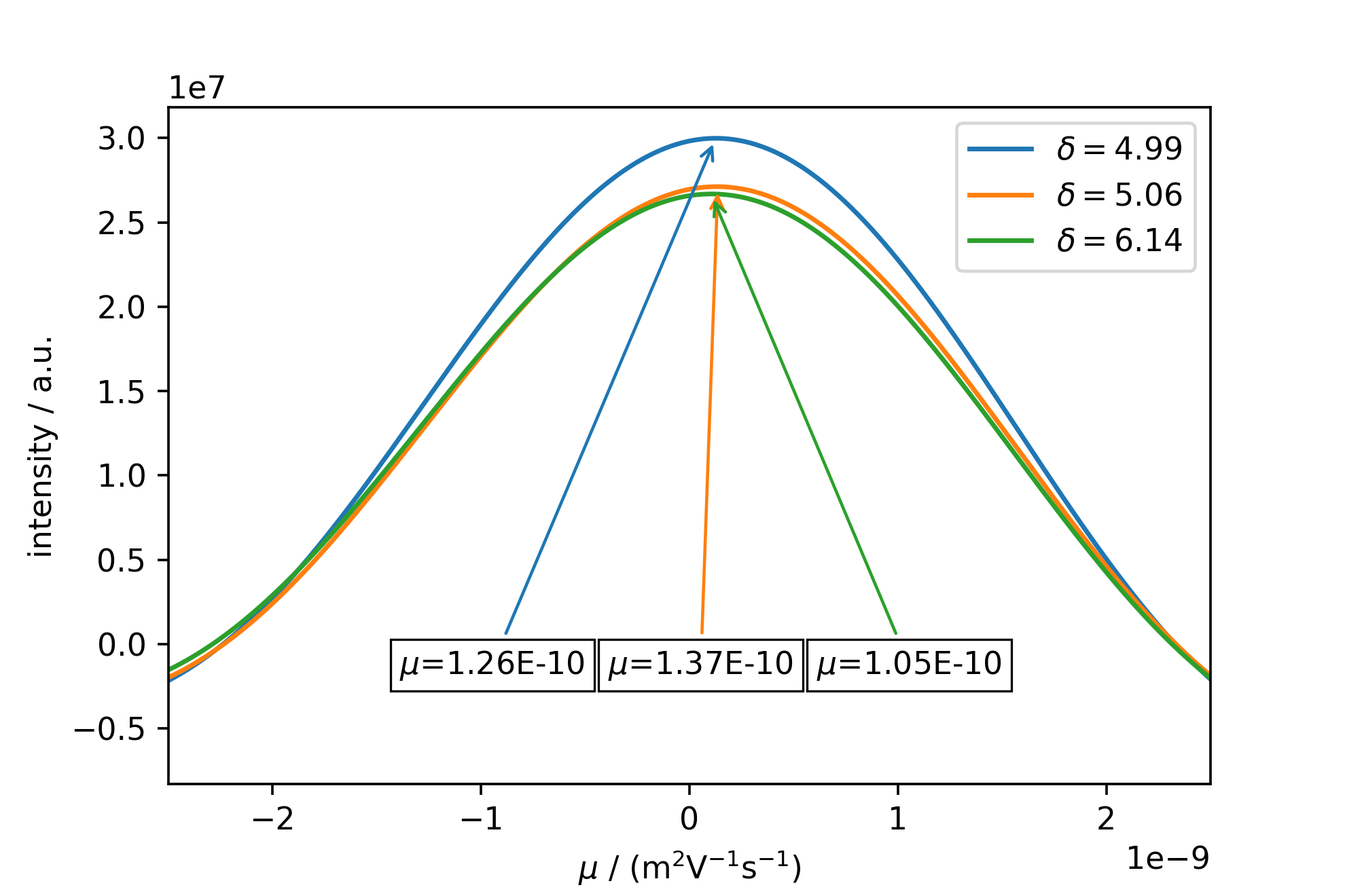
Note: Even though the mobilities of all three peaks do not completely agree, this may be the case due to an insufficient digitization of the peak, which may be corrected by a higher zerofilling in self.calc_MOSY(), but also shows the limitations of MOSY analysis on substances exhibiting only a small phase shift range. It is however very helpful for complex spectra with large phase shift-ranges and a multitude of components with different mobilities, and also has the capability to resolve a superposition of two or more mobilities modulating a single NMR resonance.
Calculating the mobility from phase data
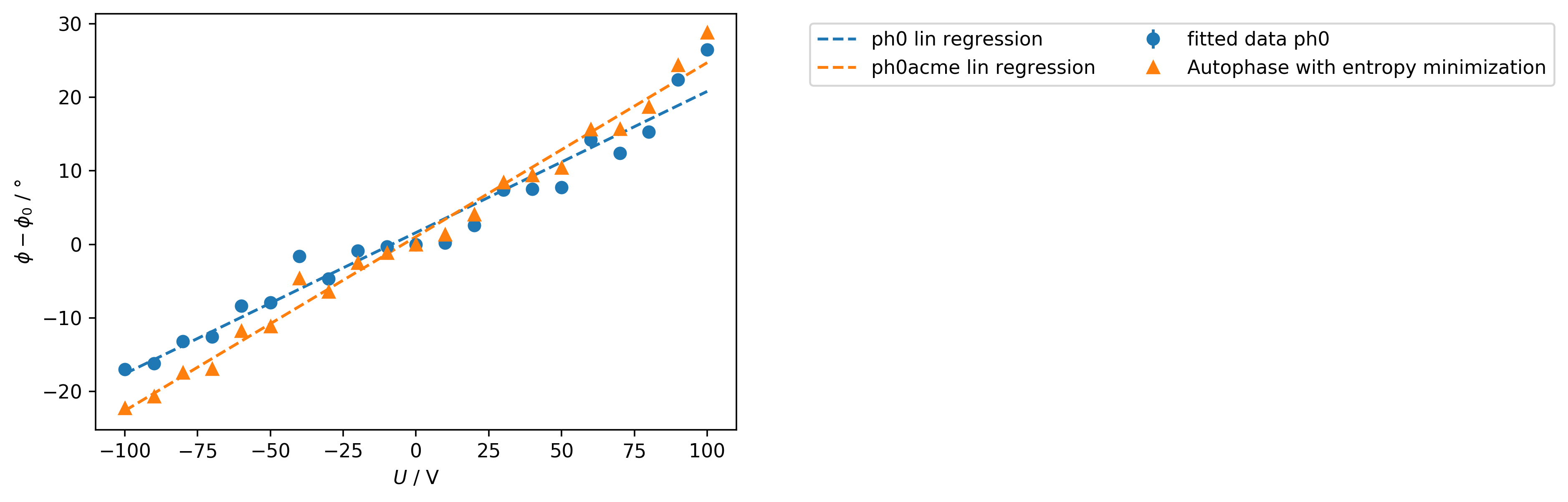
In order to calculate the mobility, a linear regression has to be performed on the phase data in the eNMR measurement object, here m. For this reason, the method self.lin_huber() is used as a robust lin. regression method using the least squares approach with a threshold epsilon, looking for outliers. Here, it is reasonable to set the threshold to 3, in order to include all data points assuming a large scattering of the phase values. Data points which are excluded from the linear regression are depicted as red dots when using self.lin_display(). y_column sets the variable to be fitted and displayed. The phase variables from the fit model are named ph0, ph1, ph2, […], while the phase variable originating from the autophase method is named ph0acme.
>>> m.lin_huber(epsilon=3, y_column='ph0')
>>> m.lin_display(y_column='ph0')
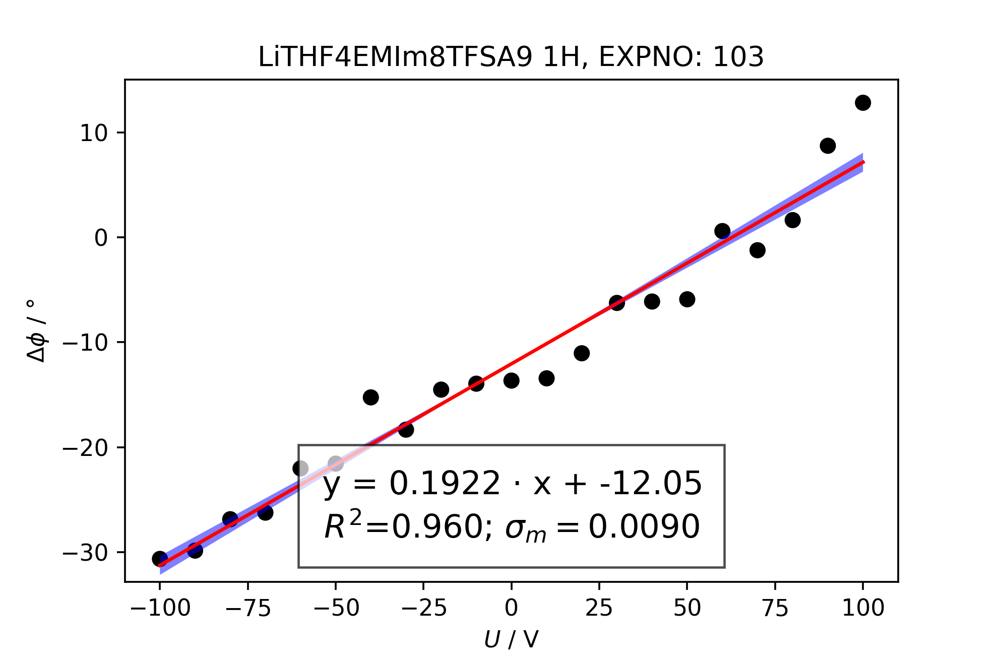
Consecutively, the mobility can be determined. Note that the electrode_distance is crucial for the calculation of the mobility. If not altered, the standard value of 2.2e-2 meters will be taken.
>>> (mobility, error) = m.mobility(y_column='ph0')
1.38E-09 (m^2/Vs) +- 6.45E-11
In order to display multiple fitted phases on top of each other use:
>>> comparephasefig = m.lin_results_display(['ph0', 'ph0acme'])
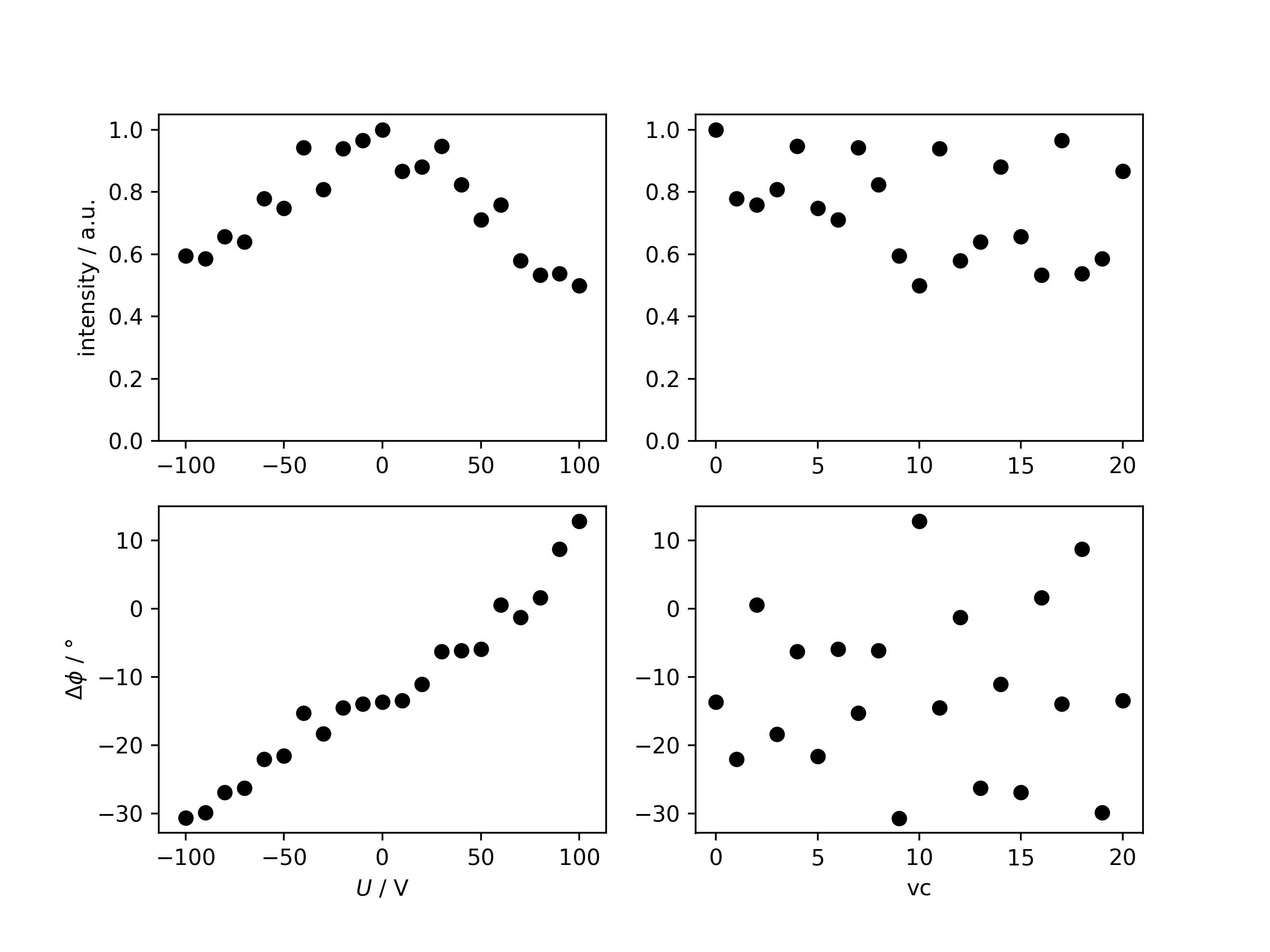
Analyzing the signal intensity after phase correction
In order to identify possible experimental artifacts, the evolution of the signal intensity can be investigated by correcting all spectra for their determined signal phase, making them fully absorptive, and consecutive integration.
>>> intensityfig, integrationresults = m.analyze_intensity(ph_var='ph0')

         U  intensity         ph
 0     0.0   1.000000 -13.653589
 1   -60.0   0.778901 -22.025162
 2    60.0   0.758279   0.597989
 3   -30.0   0.807881 -18.331584
 4    30.0   0.948111  -6.251822
 5   -50.0   0.748151 -21.568244
 6    50.0   0.711298  -5.904790
 7   -40.0   0.942212 -15.254777
 8    40.0   0.823194  -6.118121
 9  -100.0   0.595154 -30.651999
 10  100.0   0.499146  12.829012
 11  -20.0   0.940226 -14.515923
 12   70.0   0.579074  -1.227382
 13  -70.0   0.639213 -26.243095
 14   20.0   0.881509 -11.049295
 15  -80.0   0.657257 -26.869181
 16   80.0   0.533540   1.642832
 17  -10.0   0.965522 -13.948664
 18   90.0   0.537945   8.729907
 19  -90.0   0.585712 -29.861292
 20   10.0   0.866894 -13.439502
Saving and importing measurements
After evaluating an eNMR measurement, the spectral data and phase results can be stored in a .eNMRpy file.
m.save_eNMRpy(path)
In order to save only the self.eNMRraw table in excel format, use:
m.eNMRraw.to_excel(path)
Loading past results works this way:
from eNMRpy import tools

m_imported = tools.Load_eNMRpy_data('measurement_test.eNMRpy')
The loaded results can be used in almost any way, as its original measurement object. This way of loading measurements is intended to archive several evaluation versions of the same or different measurements, and load them at some time in the future for comparison or plotting reasons.